画像パート 機械学習編#
このNotebookは,情報科学演習の画像パート機械学習編に関する資料とコードをまとめたものです.
基本的には,以下の流れで進めます.
目標
機械学習に関する座学
3層ニューラルネットワークの訓練&検証
1. 目標#
機械学習編の目標は以下の3点です.
ニューラルネットワークの基礎を理解
3層ニューラルネットワークのサンプルコードを動かしてみる
3層NNの精度向上に取り組む
2. 機械学習に関する座学#
import numpy as np
import matplotlib.pyplot as plt
import japanize_matplotlib
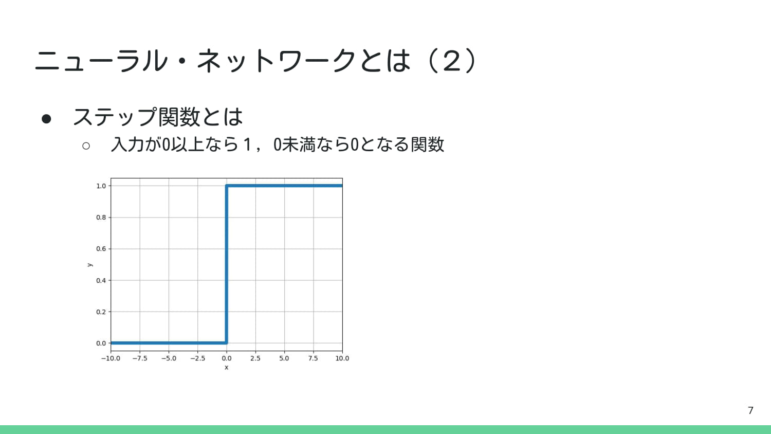
# ステップ関数(単純パーセプトロンの活性化関数)を定義
def step_function(x):
# x >= 0 なら 1.0, それ以外は 0.0 を返す
return np.where(x >= 0, 1.0, 0.0)
# x軸の範囲を生成
x = np.arange(-10.0, 10.0, 0.1)
y = step_function(x)
# グラフ描画
plt.figure(figsize=(8, 4))
plt.plot(x, y, linewidth=3)
plt.title('ステップ関数 (Step Function)')
plt.xlabel('x (入力)')
plt.ylabel('y (出力)')
plt.grid(True)
plt.yticks(np.arange(0, 1.1, 0.2))
plt.axhline(0, color='gray', linestyle='--')
plt.axvline(0, color='gray', linestyle='--')
plt.ylim(-0.1, 1.1)
plt.show()
# 出力例
print(f"入力 x=0.5 のとき,出力 y={step_function(0.5)}")
print(f"入力 x=-0.5 のとき,出力 y={step_function(-0.5)}")
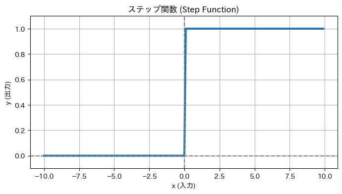
入力 x=0.5 のとき,出力 y=1.0
入力 x=-0.5 のとき,出力 y=0.0
import sys
import os
sys.path.append(os.path.abspath(os.path.join(os.getcwd(), '..')))
from util import simple_perceptron
# NumPyを使用して3x3の画像入力を定義(1を明るいピクセルとする)
input_o = np.array([
[0, 1, 0],
[1, 0, 1],
[0, 1, 0]
]).flatten() # 1次元に平坦化して入力ベクトルとする (9次元)
# NGパターン(中央に「X」パターン)の定義
input_x = np.array([
[1, 0, 1],
[0, 1, 0],
[1, 0, 1]
]).flatten()
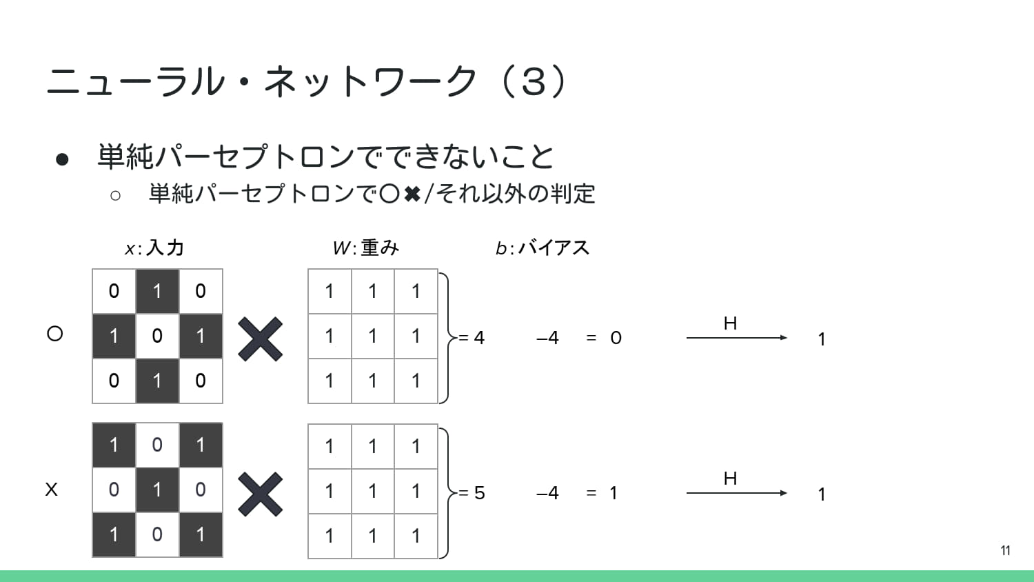
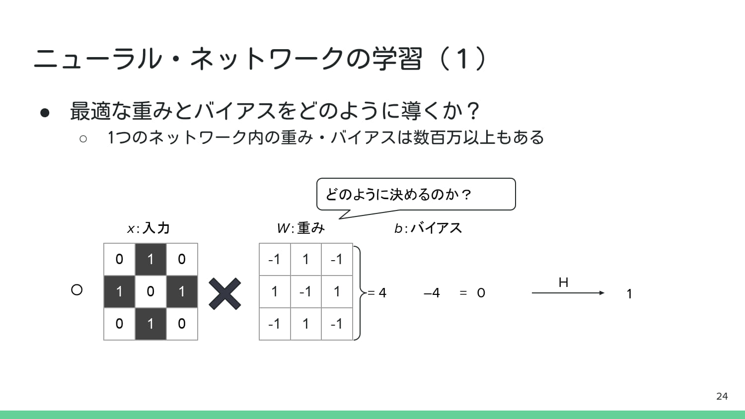
# --- 単純パーセプトロンのパラメータ (P.8の図より重みを想定) ---
# 「O」パターンに反応するような重みを定義(中央が負の値,周囲が正の値)
weight_o = np.array([
[-1, 1, -1],
[1, -1, 1],
[-1, 1, -1]
]).flatten()
bias = 4 # バイアス (b)
# 結果の表示
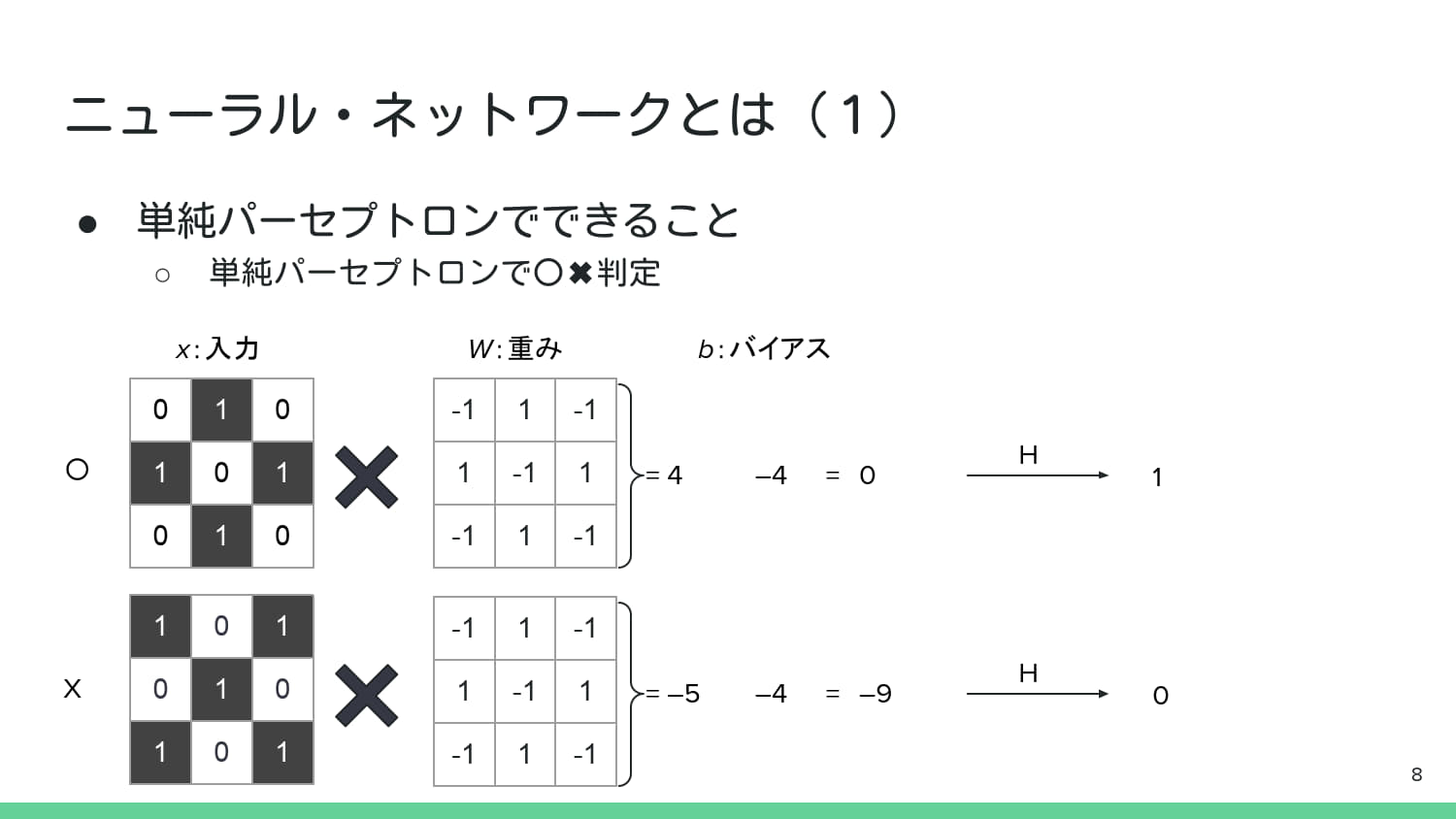
print("--- 単純パーセプトロンによる「○」判定 (P.8) ---")
# 「○」入力の判定
sum_o, net_o, output_o = simple_perceptron(input_o, weight_o, bias)
print(f"「○」入力:\n {input_o.reshape(3,3)}")
print(f"積和: {sum_o}, net_input: {net_o} (>=0? -> {net_o >= 0}), 出力 H: {output_o}")
# 「X」入力の判定 (P.8の2番目の例に相当)
sum_x, net_x, output_x = simple_perceptron(input_x, weight_o, bias)
print(f"\n「X」入力:\n {input_x.reshape(3,3)}")
print(f"積和: {sum_x}, net_input: {net_x} (>=0? -> {net_x >= 0}), 出力 H: {output_x}")
# P.8の結果では「○」に「1」を出力し,「X」に「0」を出力.
# これは,この重みとバイアスで「○」と「X」を線形分離できることを示す.
--- 単純パーセプトロンによる「○」判定 (P.8) ---
「○」入力:
 [[0 1 0]
 [1 0 1]
 [0 1 0]]
積和: 4, net_input: 0 (>=0? -> True), 出力 H: 1

「X」入力:
 [[1 0 1]
 [0 1 0]
 [1 0 1]]
積和: -5, net_input: -9 (>=0? -> False), 出力 H: 0

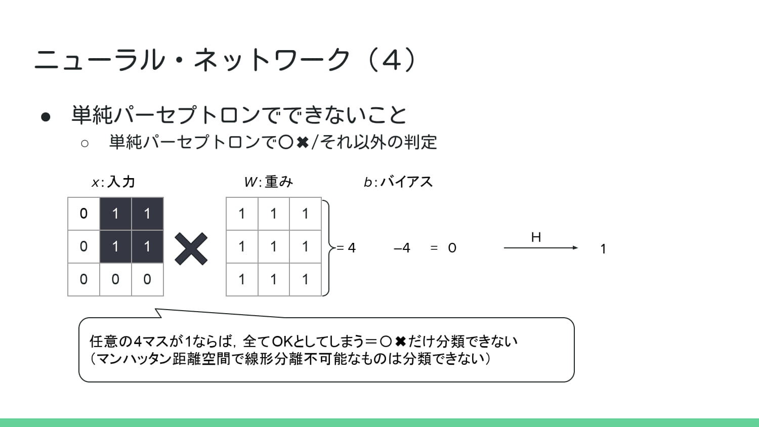
# --- P.12の線形分離不可能な例をシミュレーション ---

# 目的の重みとバイアス(P.11, P.12の図より想定)
# 周囲全体に反応するような重みを定義 (全て 1)
weight_all = np.array([
    [1, 1, 1],
    [1, 1, 1],
    [1, 1, 1]
]).flatten()
bias_p12 = -4 # バイアス (b=4)

# 入力画像1: 「○」パターン (P.11の1番目の入力)
input_o_p11 = np.array([
    [0, 1, 0],
    [1, 0, 1],
    [0, 1, 0]
]).flatten()

# 入力画像2: 「X」パターン (P.11の2番目の入力)
input_x_p11 = np.array([
    [1, 0, 1],
    [0, 1, 0],
    [1, 0, 1]
]).flatten()

# 「○」パターンの判定
sum_o_p12, net_o_p12, output_o_p12 = simple_perceptron(input_o_p11, weight_all, bias_p12)
print(f"「○」入力: \n{input_o_p11.reshape(3,3)}")
print(f"積和: {sum_o_p12}, net_input: {net_o_p12} (>=0? -> {net_o_p12 >= 0}), 出力 H: {output_o_p12}")

sum_x_p12, net_x_p12, output_x_p12 = simple_perceptron(input_x_p11, weight_all, bias_p12)
print(f"\n「X」入力: \n{input_x_p11.reshape(3,3)}")
print(f"積和: {sum_x_p12}, net_input: {net_x_p12} (>=0? -> {net_x_p12 >= 0}), 出力 H: {output_x_p12}")
「○」入力:
[[0 1 0]
 [1 0 1]
 [0 1 0]]
積和: 4, net_input: 8 (>=0? -> True), 出力 H: 1

「X」入力:
[[1 0 1]
 [0 1 0]
 [1 0 1]]
積和: 5, net_input: 9 (>=0? -> True), 出力 H: 1
# 目的の重みとバイアス(P.11, P.12の図より想定)
# 周囲全体に反応するような重みを定義 (全て 1)
weight_all = np.array([
    [1, 1, 1],
    [1, 1, 1],
    [1, 1, 1]
]).flatten()
bias_p12 = 4 # バイアス (b=4)

# 入力画像3: 「□の右半分」パターン (P.12の1番目の入力)
input_right_half_p12 = np.array([
    [0, 1, 1],
    [0, 1, 1],
    [0, 0, 0]
]).flatten()

# 入力画像4: 「上の行のみ」パターン (P.12の3番目の入力)
input_top_row_p12 = np.array([
    [1, 1, 1],
    [0, 0, 0],
    [0, 0, 0]
]).flatten()

# 入力画像5: 「適当な4マス」パターン (P.12の4番目の入力)
input_random_4_p12 = np.array([
    [1, 0, 0],
    [0, 1, 0],
    [0, 0, 1]
]).flatten()

# 入力画像6: 「全マス」パターン (P.12の5番目の入力)
input_all_p12 = np.array([
    [1, 1, 1],
    [1, 1, 1],
    [1, 1, 1]
]).flatten()

print("\n--- 線形分離不可能な例 (P.12) ---")

# 「□の右半分」パターンの判定
sum_right_p12, net_right_p12, output_right_p12 = simple_perceptron(input_right_half_p12, weight_all, bias_p12)
print(f"\n「□の右半分」入力: \n{input_right_half_p12.reshape(3,3)}")
print(f"積和: {sum_right_p12}, net_input: {net_right_p12} (>=0? -> {net_right_p12 >= 0}), 出力 H: {output_right_p12}")

# 「上の行のみ」パターンの判定
sum_top_p12, net_top_p12, output_top_p12 = simple_perceptron(input_top_row_p12, weight_all, bias_p12)
print(f"\n「上の行のみ」入力: \n{input_top_row_p12.reshape(3,3)}")
print(f"積和: {sum_top_p12}, net_input: {net_top_p12} (>=0? -> {net_top_p12 >= 0}), 出力 H: {output_top_p12}")
# 「適当な4マス」パターンの判定
sum_random_4_p12, net_random_4_p12, output_random_4_p12 = simple_perceptron(input_random_4_p12, weight_all, bias_p12)
print(f"\n「適当な4マス」入力: \n{input_random_4_p12.reshape(3,3)}")
print(f"積和: {sum_random_4_p12}, net_input: {net_random_4_p12} (>=0? -> {net_random_4_p12 >= 0}), 出力 H: {output_random_4_p12}")
# 「全マス」パターンの判定
sum_all_p12, net_all_p12, output_all_p12 = simple_perceptron(input_all_p12, weight_all, bias_p12)
print(f"\n「全マス」入力: \n{input_all_p12.reshape(3,3)}")
print(f"積和: {sum_all_p12}, net_input: {net_all_p12} (>=0? -> {net_all_p12 >= 0}), 出力 H: {output_all_p12}")
--- 線形分離不可能な例 (P.12) ---

「□の右半分」入力:
[[0 1 1]
 [0 1 1]
 [0 0 0]]
積和: 4, net_input: 0 (>=0? -> True), 出力 H: 1

「上の行のみ」入力:
[[1 1 1]
 [0 0 0]
 [0 0 0]]
積和: 3, net_input: -1 (>=0? -> False), 出力 H: 0

「適当な4マス」入力:
[[1 0 0]
 [0 1 0]
 [0 0 1]]
積和: 3, net_input: -1 (>=0? -> False), 出力 H: 0

「全マス」入力:
[[1 1 1]
 [1 1 1]
 [1 1 1]]
積和: 9, net_input: 5 (>=0? -> True), 出力 H: 1
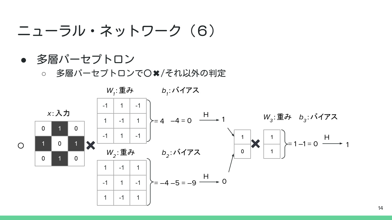
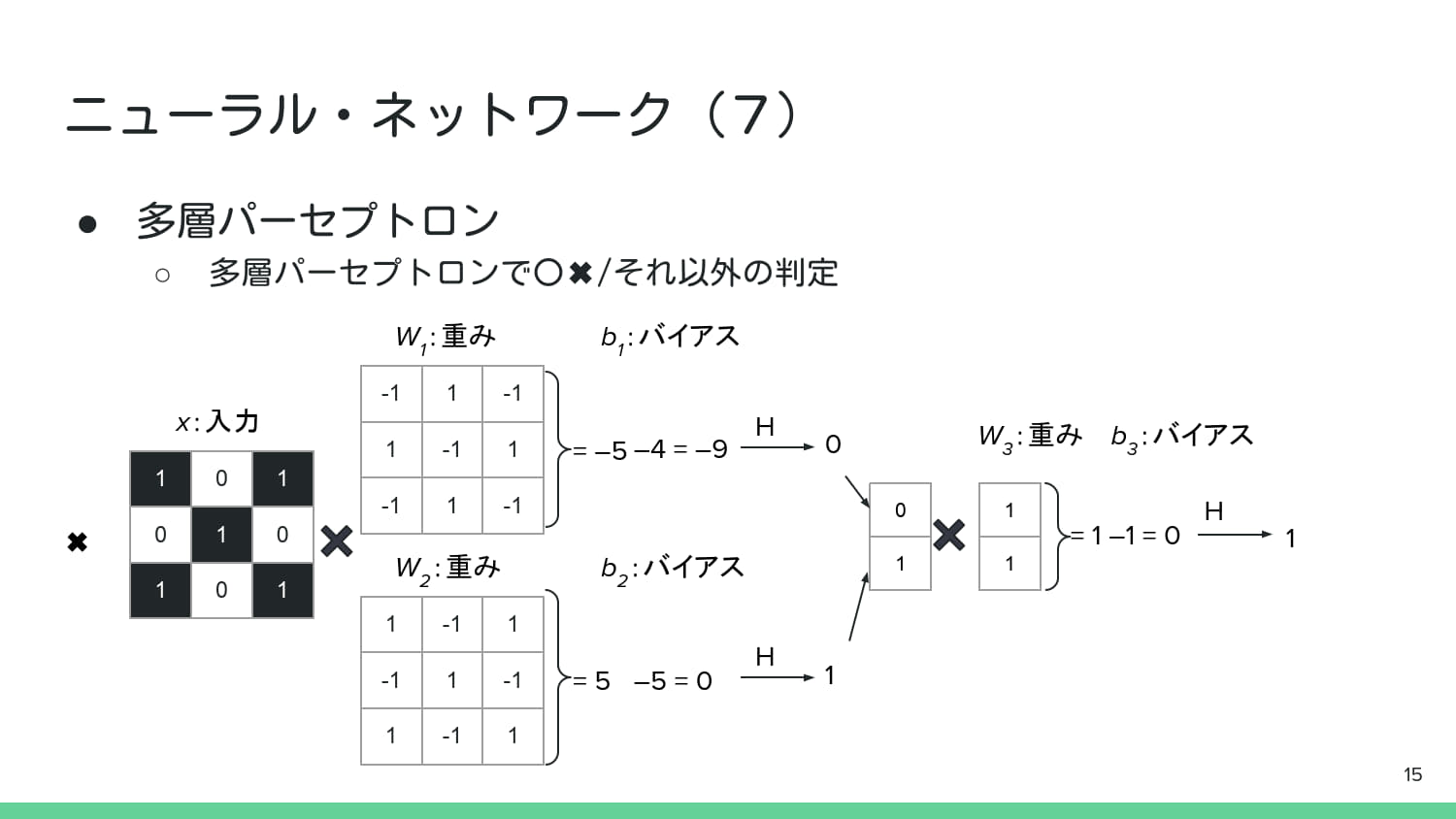
# --- P.14の多層パーセプトロンによる「○」判定のシミュレーション ---

# 入力画像1: 「○」パターン (P.14の1番目の入力)
input_o_p14 = np.array([
    [0, 1, 0],
    [1, 0, 1],
    [0, 1, 0]
]).flatten()

# 入力画像2: 「X」パターン (P.15の2番目の入力)
input_x_p15 = np.array([
    [1, 0, 1],
    [0, 1, 0],
    [1, 0, 1]
]).flatten()

# --- 第1層のパラメータ (2つの単純パーセプトロン H1, H2 に相当) ---
# H1 (P.14, W1) - 「○」パターンの特徴を検出する重み(中央が負,周囲が正)
W1 = np.array([
    [-1, 1, -1],
    [1, -1, 1],
    [-1, 1, -1]
]).flatten()
b1 = 4 # バイアス (b1)

# H2 (P.14, W2) - 「X」パターンの特徴を検出する重み(中央が正,周囲が負)
W2 = np.array([
    [1, -1, 1],
    [-1, 1, -1],
    [1, -1, 1]
]).flatten()
b2 = 5 # バイアス (b2)

# --- 第2層のパラメータ (最終出力層 H3 に相当) ---
W3 = np.array([1, 1])
b3 = 1 # バイアス (b3)

def multi_layer_perceptron_p14(input_vector):
    # --- 第1層 (中間層) ---
    # H1の計算
    sum_h1, net_h1, output_h1 = simple_perceptron(input_vector, W1, b1)

    # H2の計算
    sum_h2, net_h2, output_h2 = simple_perceptron(input_vector, W2, b2)

    # 中間層の出力ベクトル
    intermediate_output = np.array([output_h1, output_h2])

    # --- 第2層 (出力層) ---
    # H3の計算
    sum_h3, net_h3, output_h3 = simple_perceptron(intermediate_output, W3, b3)

    return output_h1, output_h2, net_h3, output_h3

# 「○」入力の判定 (P.14の例)
o_h1, o_h2, o_net_h3, o_output_h3 = multi_layer_perceptron_p14(input_o_p14)
print(f"「○」入力: \n{input_o_p14.reshape(3,3)}")
print(f"中間層 H1出力: {o_h1}, H2出力: {o_h2}")
print(f"最終層 net_input: {o_net_h3}, 出力 H3: {o_output_h3}")

# 「X」入力の判定 (P.15の例)
x_h1, x_h2, x_net_h3, x_output_h3 = multi_layer_perceptron_p14(input_x_p15)
print(f"\n「X」入力: \n{input_x_p15.reshape(3,3)}")
print(f"中間層 H1出力: {x_h1}, H2出力: {x_h2}")
print(f"最終層 net_input: {x_net_h3}, 出力 H3: {x_output_h3}")

# P.14, P.15の図に対応した結果が得られ,「○」と「X」を正しく分類できている.
「○」入力:
[[0 1 0]
 [1 0 1]
 [0 1 0]]
中間層 H1出力: 1, H2出力: 0
最終層 net_input: 0, 出力 H3: 1

「X」入力:
[[1 0 1]
 [0 1 0]
 [1 0 1]]
中間層 H1出力: 0, H2出力: 1
最終層 net_input: 0, 出力 H3: 1
# 入力画像3: 「□の右半分」パターン (P.12の1番目の入力)
input_right_half_p12 = np.array([
    [0, 1, 1],
    [0, 1, 1],
    [0, 0, 0]
]).flatten()

# 入力画像4: 「上の行のみ」パターン (P.12の3番目の入力)
input_top_row_p12 = np.array([
    [1, 1, 1],
    [0, 0, 0],
    [0, 0, 0]
]).flatten()

# 入力画像5: 「適当な4マス」パターン (P.12の4番目の入力)
input_random_4_p12 = np.array([
    [1, 0, 0],
    [0, 1, 0],
    [0, 0, 1]
]).flatten()

# 入力画像6: 「全マス」パターン (P.12の5番目の入力)
input_all_p12 = np.array([
    [1, 1, 1],
    [1, 1, 1],
    [1, 1, 1]
]).flatten()

# 多重パーセプトロンでの判定例

output_h1_right, output_h2_right, net_h3_right, output_h3_right = multi_layer_perceptron_p14(input_right_half_p12)
print(f"\n「□の右半分」入力: \n{input_right_half_p12.reshape(3,3)}")
print(f"中間層 H1出力: {output_h1_right}, H2出力: {output_h2_right}")
print(f"最終層 net_input: {net_h3_right}, 出力 H3: {output_h3_right}")

output_h1_top, output_h2_top, net_h3_top, output_h3_top = multi_layer_perceptron_p14(input_top_row_p12)
print(f"\n「上の行のみ」入力: \n{input_top_row_p12.reshape(3,3)}")
print(f"中間層 H1出力: {output_h1_top}, H2出力: {output_h2_top}")
print(f"最終層 net_input: {net_h3_top}, 出力 H3: {output_h3_top}")

output_h1_random, output_h2_random, net_h3_random, output_h3_random = multi_layer_perceptron_p14(input_random_4_p12)
print(f"\n「適当な4マス」入力: \n{input_random_4_p12.reshape(3,3)}")
print(f"中間層 H1出力: {output_h1_random}, H2出力: {output_h2_random}")
print(f"最終層 net_input: {net_h3_random}, 出力 H3: {output_h3_random}")

output_h1_all, output_h2_all, net_h3_all, output_h3_all = multi_layer_perceptron_p14(input_all_p12)
print(f"\n「全マス」入力: \n{input_all_p12.reshape(3,3)}")
print(f"中間層 H1出力: {output_h1_all}, H2出力: {output_h2_all}")
print(f"最終層 net_input: {net_h3_all}, 出力 H3: {output_h3_all}")
「□の右半分」入力:
[[0 1 1]
 [0 1 1]
 [0 0 0]]
中間層 H1出力: 0, H2出力: 0
最終層 net_input: -1, 出力 H3: 0

「上の行のみ」入力:
[[1 1 1]
 [0 0 0]
 [0 0 0]]
中間層 H1出力: 0, H2出力: 0
最終層 net_input: -1, 出力 H3: 0

「適当な4マス」入力:
[[1 0 0]
 [0 1 0]
 [0 0 1]]
中間層 H1出力: 0, H2出力: 0
最終層 net_input: -1, 出力 H3: 0

「全マス」入力:
[[1 1 1]
 [1 1 1]
 [1 1 1]]
中間層 H1出力: 0, H2出力: 0
最終層 net_input: -1, 出力 H3: 0
演習課題①:3*3内の特定の直線判定パーセプトロンの実装せよ#
概要#
3×3 の二値画像(0 または 1)を入力とし,特定の縦・横・斜めの直線パターンを検出するパーセプトロンを実装せよ.
「特定直線パターン」とは,以下に示す入力パターン例のうち,縦線(中央),横線(中央),斜め線(左上→右下)の3種類を指す.
サンプルコード内のW_FILTER(重み),B_BIAS(バイアス)を適切に設定し,テストケースを突破することを目標とする.
入力パターン例#
種類 |
3×3 パターン |
|---|---|
縦線(中央) |
|
横線(中央) |
|
斜め線(左上→右下) |
|
L字(だめな例1) |
|
点(だめな例2) |
|
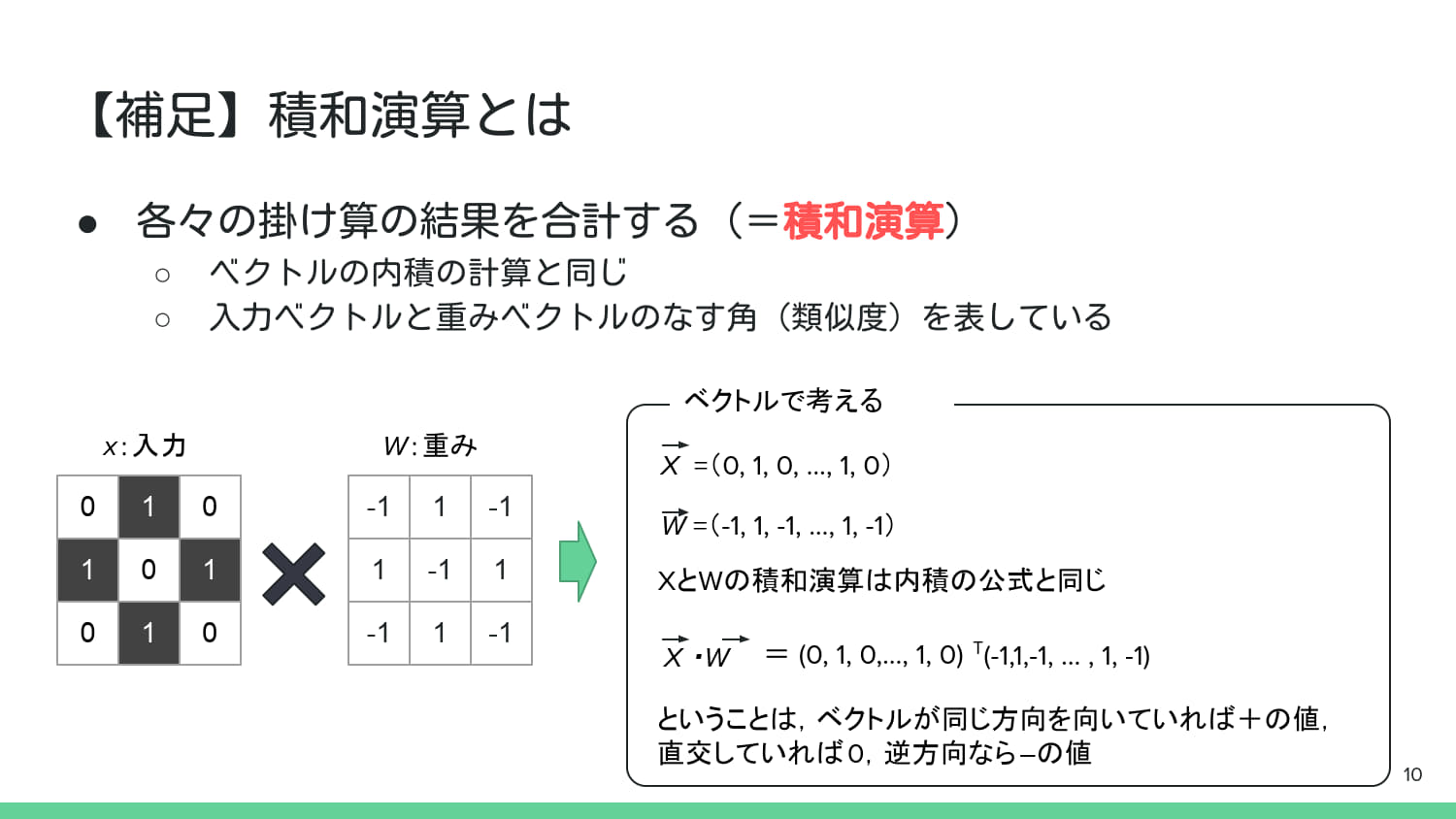
from util import get_test_patterns, visualize_filters_and_tests
import numpy as np
import japanize_matplotlib

# --- 編集する部分 ---
W_H_3X3_List = [
    np.array([[1, -1, -1],
              [1, -1, -1],
              [1, -1, -1]]),
    np.array([[-1, -1, -1],
              [-1, -1, -1],
              [-1, -1, -1]]),
    np.array([[-1, -1, -1],
              [-1, -1, -1],
              [-1, -1, -1]])
]

W_H = np.array([w.flatten() for w in W_H_3X3_List])
B_H = np.array([2.5, 2.5, 2.5])

W_OUT = np.array([1, 1, 1])
B_OUT = 0.5

# --- テストパターンを取得 ---
TEST_PATTERNS = get_test_patterns()

# --- 可視化 ---
visualize_filters_and_tests(W_H, B_H, W_OUT, B_OUT, TEST_PATTERNS)
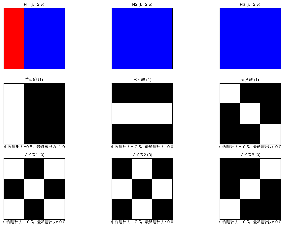
--- 最終判定結果 ---
垂直線 (1): 判定結果 = 1
水平線 (1): 判定結果 = 0
対角線 (1): 判定結果 = 0
ノイズ1 (0): 判定結果 = 0
ノイズ2 (0): 判定結果 = 0
ノイズ3 (0): 判定結果 = 0
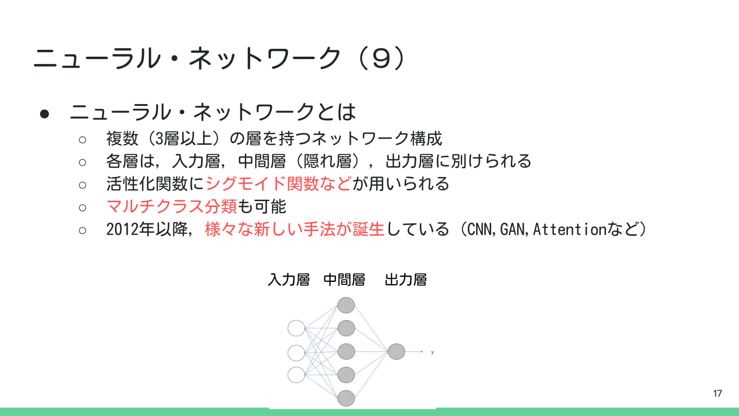
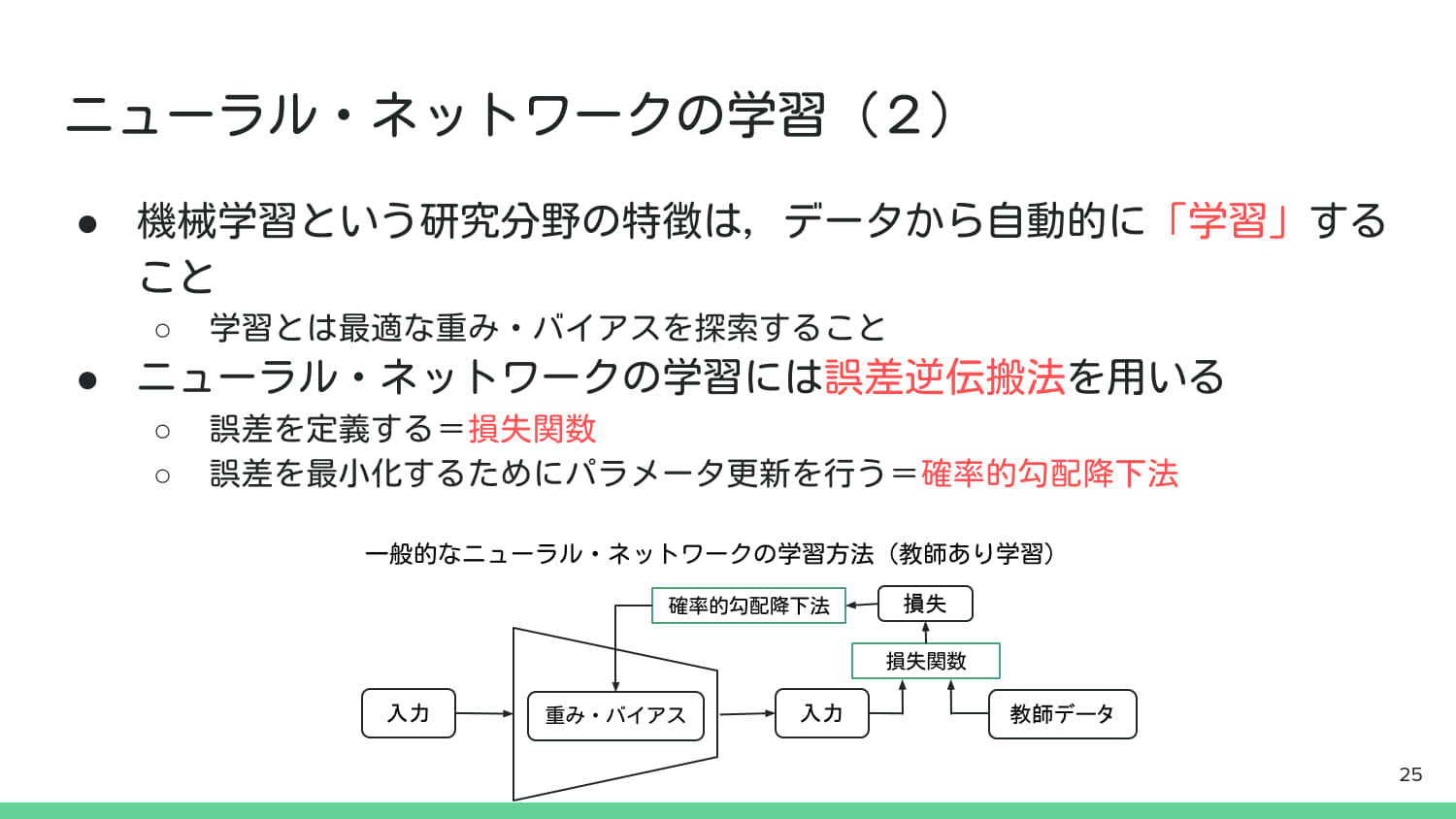
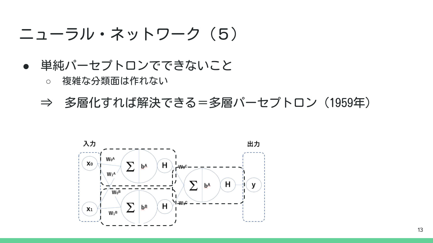
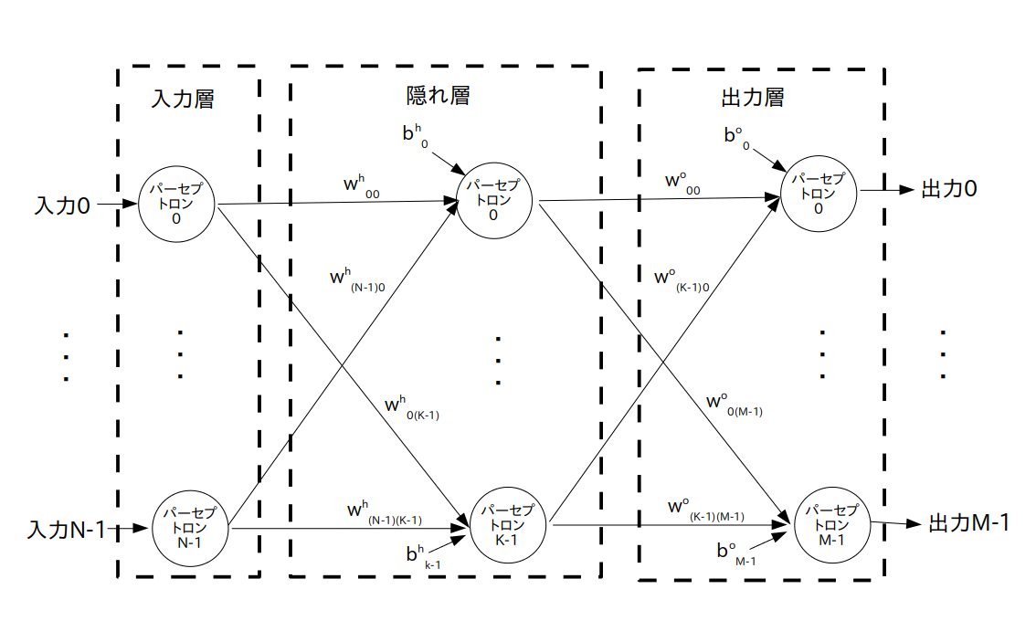
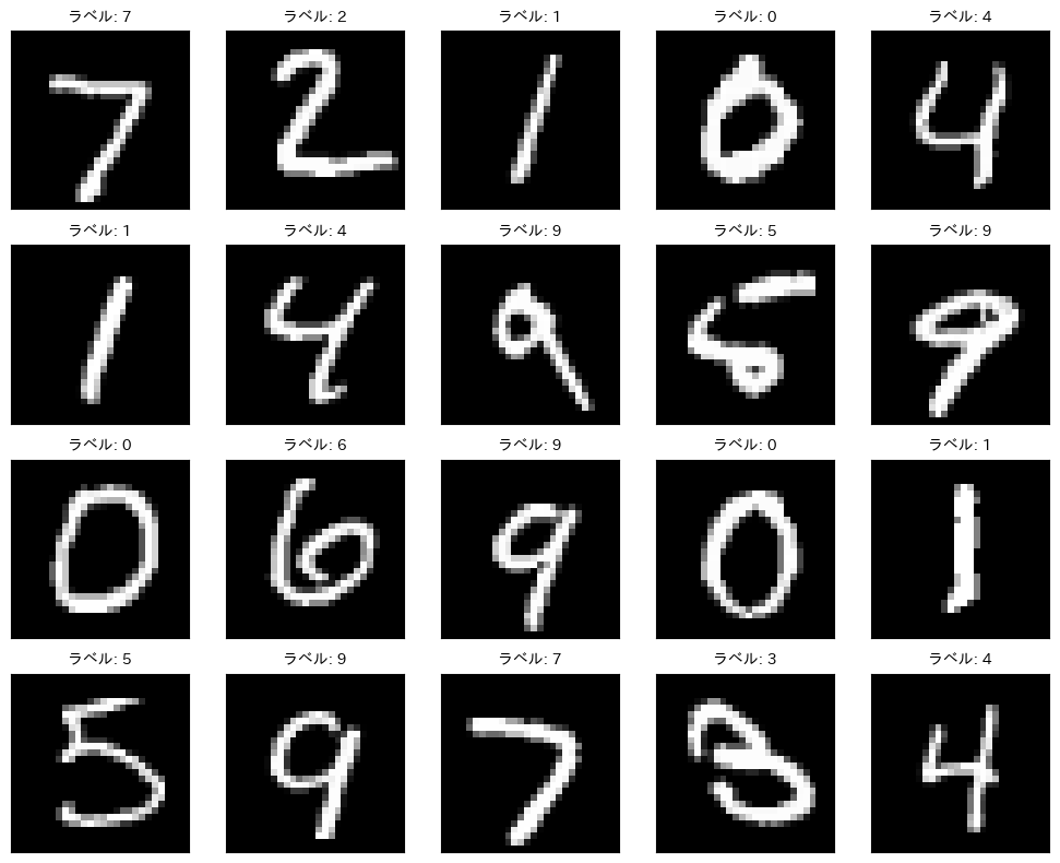
3. 3層ニューラルネットワーク(MLP)の訓練&検証#
最も単純な構造のMLPを定義し,MNISTデータを用いて学習と検証を行う.
MNIST:手書き数字の画像データセット.0から9までの数字が含まれる.
学習後は,学習の進み具合やテスト画像の予測結果,混同行列の可視化などを行う.
また,MLPのハイパーパラメータを変更して,学習結果に与える影響を確認する.
以下イメージ図.
import torch
import torch.nn as nn
import torch.optim as optim
import torch.nn.functional as F
from torchvision import datasets, transforms
from torch.utils.data import DataLoader
from sklearn.metrics import confusion_matrix
import seaborn as sns

# GPU利用設定
device = torch.device("cuda" if torch.cuda.is_available() else "cpu")
print("使用デバイス:", device)

# データ変換(Tensor化+正規化)
transform = transforms.Compose([
    transforms.ToTensor(),
    transforms.Normalize((0.5,), (0.5,))
])

# MNISTのダウンロード&読み込み
train_dataset = datasets.MNIST(root="./data", train=True, download=True, transform=transform)
test_dataset = datasets.MNIST(root="./data", train=False, download=True, transform=transform)

train_loader = DataLoader(train_dataset, batch_size=64, shuffle=True)
test_loader = DataLoader(test_dataset, batch_size=1000, shuffle=False)
使用デバイス: cuda
Downloading http://yann.lecun.com/exdb/mnist/train-images-idx3-ubyte.gz
Failed to download (trying next):
HTTP Error 404: Not Found

Downloading https://ossci-datasets.s3.amazonaws.com/mnist/train-images-idx3-ubyte.gz
Downloading https://ossci-datasets.s3.amazonaws.com/mnist/train-images-idx3-ubyte.gz to ./data/MNIST/raw/train-images-idx3-ubyte.gz
100.0%
Extracting ./data/MNIST/raw/train-images-idx3-ubyte.gz to ./data/MNIST/raw

Downloading http://yann.lecun.com/exdb/mnist/train-labels-idx1-ubyte.gz
Failed to download (trying next):
HTTP Error 404: Not Found

Downloading https://ossci-datasets.s3.amazonaws.com/mnist/train-labels-idx1-ubyte.gz
Downloading https://ossci-datasets.s3.amazonaws.com/mnist/train-labels-idx1-ubyte.gz to ./data/MNIST/raw/train-labels-idx1-ubyte.gz
100.0%
Extracting ./data/MNIST/raw/train-labels-idx1-ubyte.gz to ./data/MNIST/raw

Downloading http://yann.lecun.com/exdb/mnist/t10k-images-idx3-ubyte.gz
Failed to download (trying next):
HTTP Error 404: Not Found

Downloading https://ossci-datasets.s3.amazonaws.com/mnist/t10k-images-idx3-ubyte.gz
Downloading https://ossci-datasets.s3.amazonaws.com/mnist/t10k-images-idx3-ubyte.gz to ./data/MNIST/raw/t10k-images-idx3-ubyte.gz
100.0%
Extracting ./data/MNIST/raw/t10k-images-idx3-ubyte.gz to ./data/MNIST/raw

Downloading http://yann.lecun.com/exdb/mnist/t10k-labels-idx1-ubyte.gz
Failed to download (trying next):
HTTP Error 404: Not Found

Downloading https://ossci-datasets.s3.amazonaws.com/mnist/t10k-labels-idx1-ubyte.gz
Downloading https://ossci-datasets.s3.amazonaws.com/mnist/t10k-labels-idx1-ubyte.gz to ./data/MNIST/raw/t10k-labels-idx1-ubyte.gz
100.0%
Extracting ./data/MNIST/raw/t10k-labels-idx1-ubyte.gz to ./data/MNIST/raw
# MNISTの画像を10例表示
import matplotlib.pyplot as plt
fig, axes = plt.subplots(4, 5, figsize=(10, 8))
for i, (img, label) in enumerate(test_dataset):
    if i >= 20:
        break
    ax = axes[i // 5, i % 5]
    ax.imshow(img.squeeze(), cmap='gray')
    ax.set_title(f"ラベル: {label}", fontsize=10)
    ax.set_xticks([])
    ax.set_yticks([])
plt.tight_layout()
plt.show()
# 3層NNのモデルクラスを定義 (入力層、隠れ層、出力層の3層)
class ThreeLayerNN(nn.Module):
    # コンストラクタ: ネットワークの構造を定義する
    def __init__(self):
        super(ThreeLayerNN, self).__init__()

        # MNIST画像は28x28ピクセルで、1チャンネル(グレースケール)
        # 入力層のノード数(特徴量の総数)は 28 * 28 = 784
        input_size = 28 * 28
        # 隠れ層のノード数(ハイパーパラメータとして自由に設定可能。ここでは512に設定)
        hidden_size = 16
        # 出力層のノード数(MNISTは0-9の10クラス分類なので10)
        output_size = 10

        # 1. 入力層 -> 隠れ層1 (全結合層: Linear)
        # nn.Linear(入力サイズ, 出力サイズ)
        self.fc1 = nn.Linear(input_size, hidden_size)

        # 2. 隠れ層1 -> 隠れ層2 (もう一つの全結合層)
        self.fc2 = nn.Linear(hidden_size, hidden_size)

        # 3. 隠れ層2 -> 出力層
        self.fc3 = nn.Linear(hidden_size, output_size)

    # 順伝播の処理を定義する
    def forward(self, x):
        # 画像データを全結合層に通す前に、1次元に平坦化(Flatten)する必要がある
        # x.size(0)はバッチサイズ。-1を指定することで、残りの次元を自動で計算(28*28)
        # 例: (64, 1, 28, 28) -> (64, 784)
        x = x.view(x.size(0), -1)

        # 隠れ層1: 全結合層(fc1)の後にReLU活性化関数を適用
        x = F.relu(self.fc1(x))

        # 隠れ層2: 全結合層(fc2)の後にReLU活性化関数を適用
        x = F.relu(self.fc2(x))

        # 出力層: 全結合層(fc3)を適用。活性化関数は損失関数(CrossEntropyLoss)に含まれるため、ここでは適用しない
        x = self.fc3(x)

        return x

# モデルのインスタンス化とデバイスへの転送
model = ThreeLayerNN().to(device)
print(model)
ThreeLayerNN(
  (fc1): Linear(in_features=784, out_features=16, bias=True)
  (fc2): Linear(in_features=16, out_features=16, bias=True)
  (fc3): Linear(in_features=16, out_features=10, bias=True)
)
def train(model, loader, optimizer, criterion):
    """モデルを訓練する関数"""
    model.train() # モデルを訓練モードに設定
    total_loss = 0
    for images, labels in loader:
        images, labels = images.to(device), labels.to(device) # データをデバイスへ転送

        optimizer.zero_grad() # 勾配をゼロにリセット
        outputs = model(images) # 順伝播: 入力から出力を計算
        loss = criterion(outputs, labels) # 損失(誤差)を計算
        loss.backward() # 誤差逆伝播: 勾配を計算
        optimizer.step() # パラメータ(重みとバイアス)を更新

        total_loss += loss.item()
    return total_loss / len(loader)

def test(model, loader, criterion):
    """モデルを評価する関数"""
    model.eval() # モデルを評価モードに設定(Dropoutなどが無効になる)
    correct = 0
    total_loss = 0
    # 勾配計算をしない
    with torch.no_grad():
        for images, labels in loader:
            images, labels = images.to(device), labels.to(device)
            outputs = model(images)
            loss = criterion(outputs, labels)
            total_loss += loss.item()
            pred = outputs.argmax(dim=1) # 最大値のインデックス(予測クラス)を取得
            correct += pred.eq(labels).sum().item() # 正解数をカウント
    acc = correct / len(loader.dataset) # 正解率を計算
    return total_loss / len(loader), acc

# 学習履歴を記録するリスト
train_losses, test_losses, test_accs = [], [], []

# 損失関数: nn.CrossEntropyLoss()は分類問題で一般的に使用される
criterion = nn.CrossEntropyLoss()
# 最適化アルゴリズム: Adamを使用(lr=0.001は学習率)
optimizer = optim.Adam(model.parameters(), lr=0.001)

# 学習ループ
num_epochs = 10
for epoch in range(num_epochs):
    train_loss = train(model, train_loader, optimizer, criterion)
    test_loss, test_acc = test(model, test_loader, criterion)
    train_losses.append(train_loss)
    test_losses.append(test_loss)
    test_accs.append(test_acc)
    print(f"Epoch {epoch+1}: TrainLoss={train_loss:.4f}, TestLoss={test_loss:.4f}, TestAcc={test_acc*100:.2f}%")
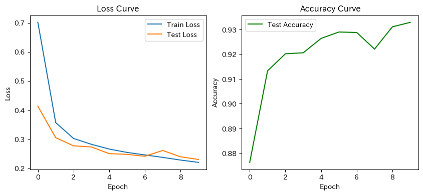
Epoch 1: TrainLoss=0.7016, TestLoss=0.4130, TestAcc=87.63%
Epoch 2: TrainLoss=0.3564, TestLoss=0.3045, TestAcc=91.33%
Epoch 3: TrainLoss=0.3019, TestLoss=0.2765, TestAcc=92.02%
Epoch 4: TrainLoss=0.2817, TestLoss=0.2726, TestAcc=92.06%
Epoch 5: TrainLoss=0.2654, TestLoss=0.2497, TestAcc=92.64%
Epoch 6: TrainLoss=0.2538, TestLoss=0.2471, TestAcc=92.90%
Epoch 7: TrainLoss=0.2452, TestLoss=0.2406, TestAcc=92.88%
Epoch 8: TrainLoss=0.2367, TestLoss=0.2605, TestAcc=92.21%
Epoch 9: TrainLoss=0.2275, TestLoss=0.2387, TestAcc=93.11%
Epoch 10: TrainLoss=0.2196, TestLoss=0.2296, TestAcc=93.29%
# 学習曲線の描画
plt.figure(figsize=(10,4))
plt.subplot(1,2,1)
plt.plot(train_losses, label="Train Loss")
plt.plot(test_losses, label="Test Loss")
plt.title("Loss Curve")
plt.xlabel("Epoch")
plt.ylabel("Loss")
plt.legend()

plt.subplot(1,2,2)
plt.plot(test_accs, label="Test Accuracy", color='green')
plt.title("Accuracy Curve")
plt.xlabel("Epoch")
plt.ylabel("Accuracy")
plt.legend()
plt.show()
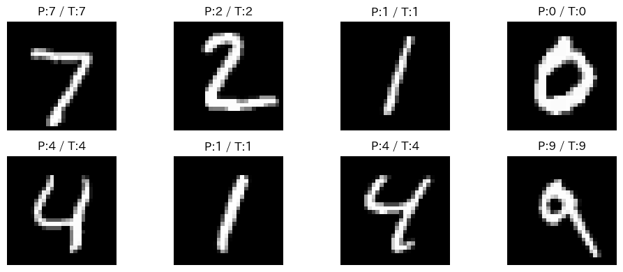
# 予測例表示
model.eval()
images, labels = next(iter(test_loader))
images, labels = images.to(device), labels.to(device)
outputs = model(images)
preds = outputs.argmax(dim=1)

plt.figure(figsize=(10,4))
for i in range(8):
    plt.subplot(2,4,i+1)
    plt.imshow(images[i].cpu().squeeze(), cmap="gray")
    plt.title(f"P:{preds[i].item()} / T:{labels[i].item()}")
    plt.axis("off")
plt.tight_layout()
plt.show()

# 全テストデータに対して予測
all_preds, all_labels = [], []
model.eval()
with torch.no_grad():
    for images, labels in test_loader:
        images, labels = images.to(device), labels.to(device)
        outputs = model(images)
        preds = outputs.argmax(dim=1)
        all_preds.extend(preds.cpu().numpy())
        all_labels.extend(labels.cpu().numpy())

# 混同行列
cm = confusion_matrix(all_labels, all_preds)
plt.figure(figsize=(8,6))
sns.heatmap(cm, annot=True, fmt="d", cmap="Blues")
plt.title("Confusion Matrix for MNIST")
plt.xlabel("Predicted")
plt.ylabel("True")
plt.show()

# 最終精度
test_loss, test_acc = test(model, test_loader, criterion)
print(f"Test Loss: {test_loss:.4f}, Test Accuracy: {test_acc*100:.2f}%")
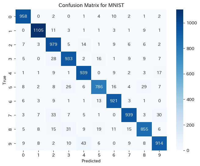
Test Loss: 0.2296, Test Accuracy: 93.29%
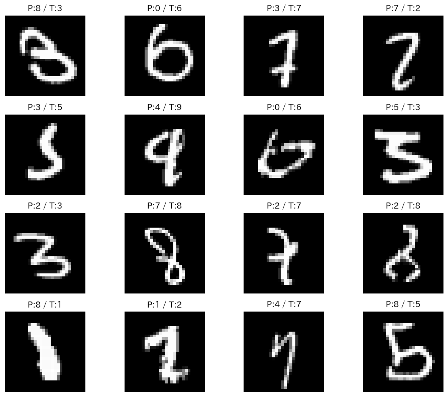
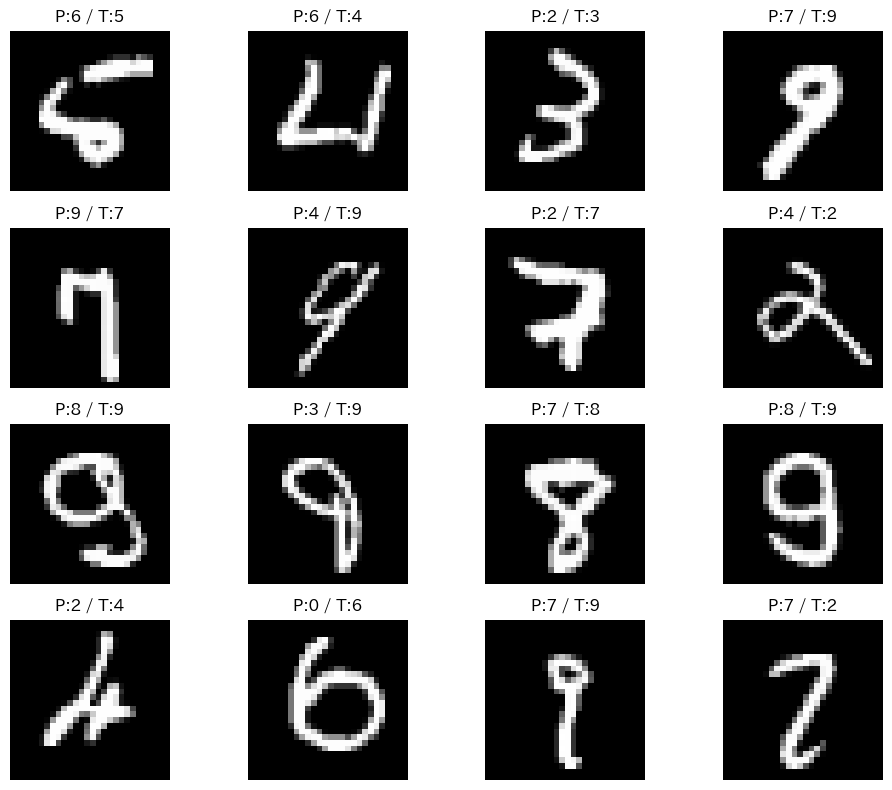
# 予測失敗した例の表示
incorrect_indices = [i for i, (p, t) in enumerate(zip(all_preds, all_labels)) if p != t]
plt.figure(figsize=(10,8))
for i, idx in enumerate(incorrect_indices[:16]):
    img, label = test_dataset[idx]
    plt.subplot(4,4,i+1)
    plt.imshow(img.squeeze(), cmap="gray")
    plt.title(f"P:{all_preds[idx]} / T:{label}")
    plt.axis("off")
plt.tight_layout()
plt.show()
演習課題②:分類精度0.99以上のCNNを構築せよ#
概要#
本課題では, PyTorch を用いて手書き数字データセット(MNIST)の分類を行う全結合型の3層ニューラルネットワーク(MLP)を構築する.
サンプルコードを参考にモデルを実装し, 訓練・検証を通して分類精度(Accuracy)0.99以上を達成することを目標とする.
手順#
MLPモデルの実装
サンプルコードを参考に, 3層ニューラルネットワークを実装する.
訓練・検証
サンプルコードを参考に, MNISTデータセットを用いてモデルの訓練・検証を行う.
精度向上のための工夫を実施
モデル構造の変更
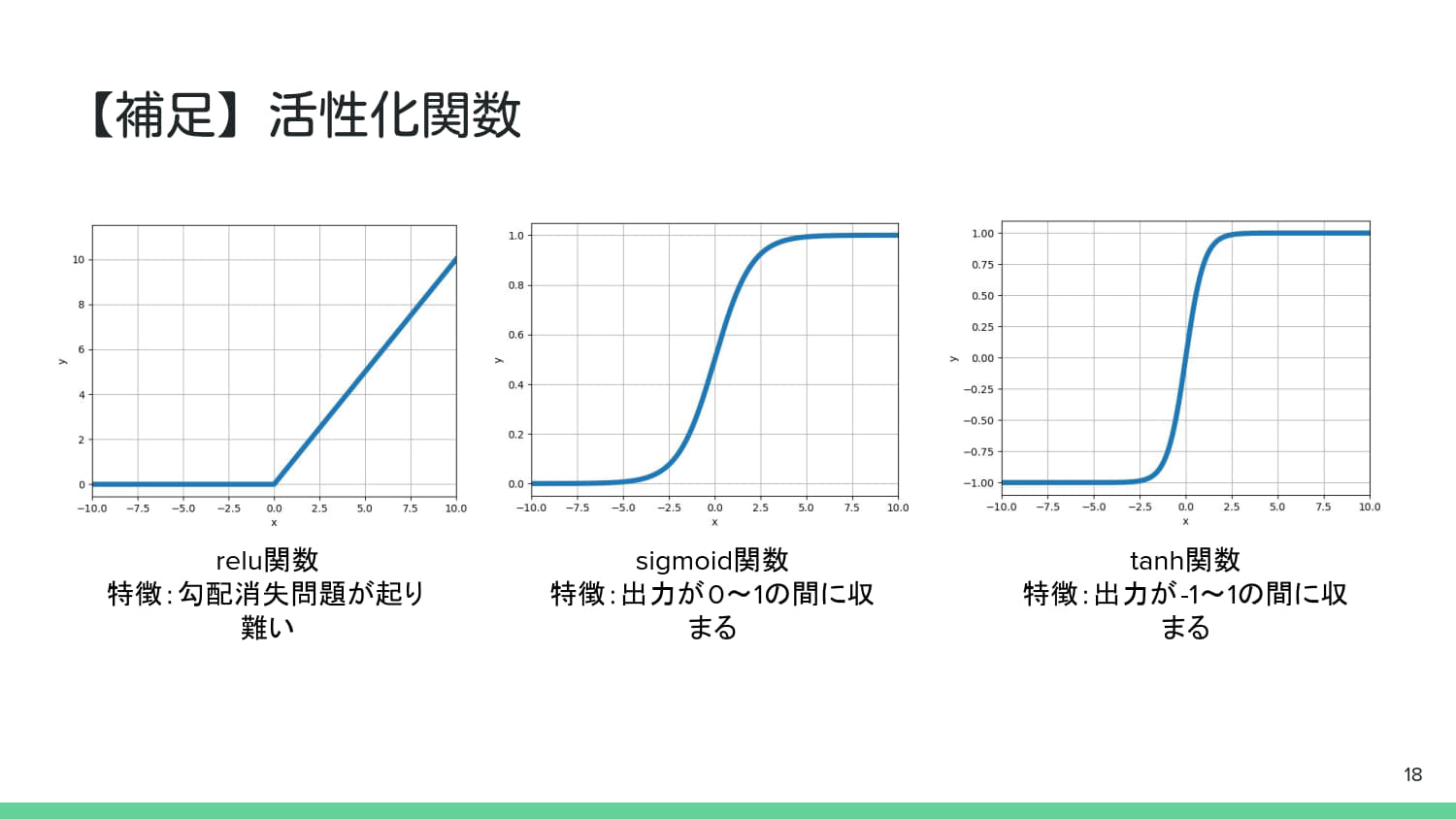
層の数,ノード数,活性化関数(ReLu,LeakyReLu,GELU等)を変更する…etc
学習パラメータの変更
epoch数,学習率,バッチサイズ,最適化手法(SGD,Adam,RMSprop等)を変更する…etc
データ拡張の導入
回転,平行移動,拡大縮小,ノイズ付加など…etc
前回の画像処理パートでやった内容が参考になるかも?
その他
正則化項(Dropout,BatchNorm等)の導入,重み初期化や学習率減衰の工夫,early stoppingの導入…etc
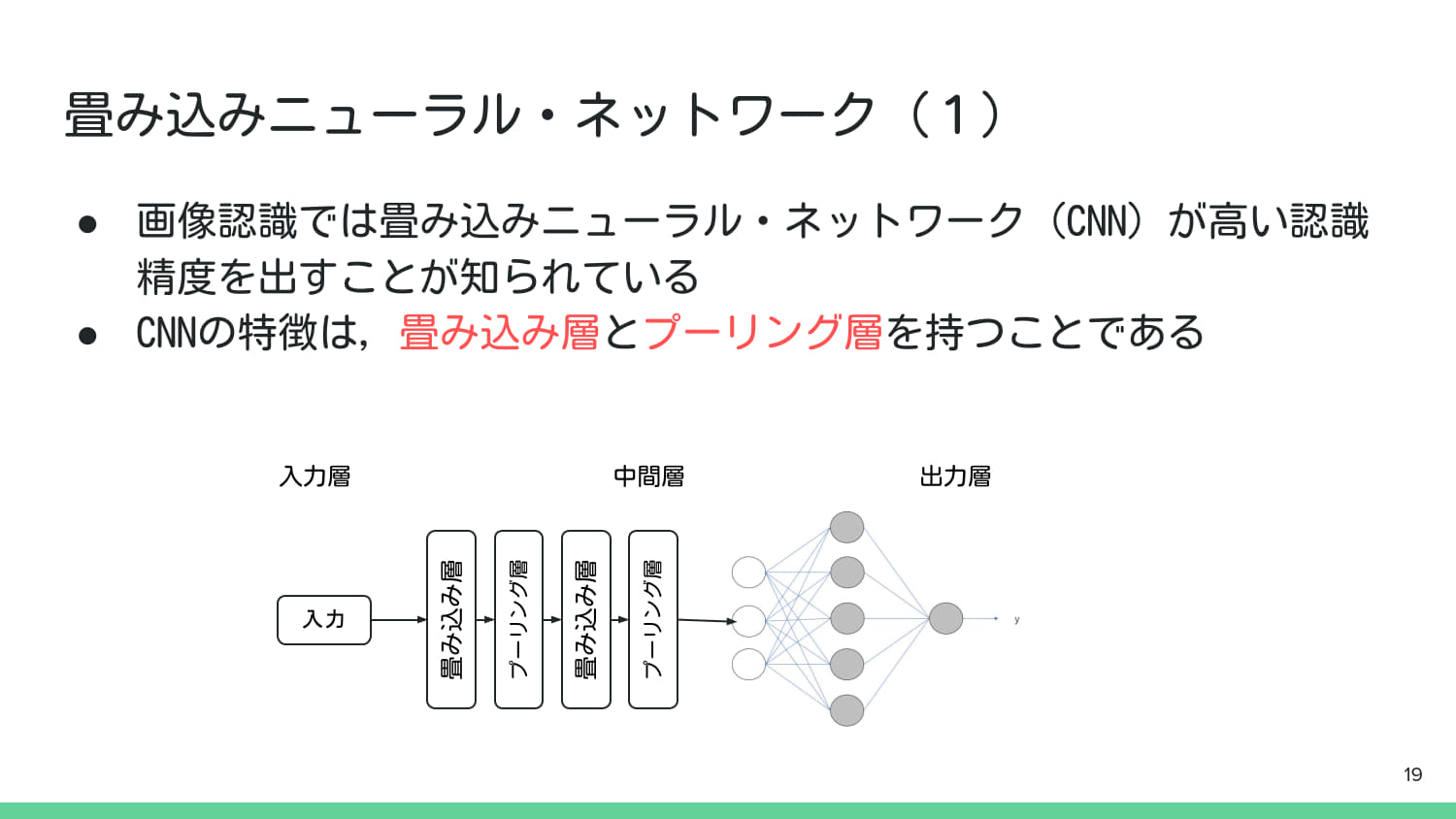
CNNモデルの構築(任意課題)
さらに高精度を目指す場合は, 畳み込みニューラルネットワーク(CNN)を構築してみるのも良い.
多分MLPより精度がでやすいはず.
資料末尾にCNNのサンプルコードを掲載しているので, 参考にしてほしい.
発表#
次回の情報科学演習までに, 改善したモデルの内容と精度に関して, 3〜5分程度のプレゼンテーション資料を準備すること.
工夫点
モデル構造
学習パラメータ
データ拡張
精度とその分析
最終精度
学習曲線(損失,精度)
混同行列
幾何学的画像拡張のサンプルコード#
import torch
import numpy as np
import cv2 # 幾何学的変換の行列(アフィン行列)計算に使用
import matplotlib.pyplot as plt
from torchvision import datasets, transforms
import random
from util import display_transforms

# ===================================================================
# 共通データセット準備(ラベル指定機能を追加)
# ===================================================================

# PIL Image形式で画像をロード(生の画像データが必要なため)
mnist_dataset = datasets.MNIST(root="./data", train=False, download=True, transform=None)

TARGET_LABEL = 6 # 例: '8'の画像を取得

# 指定したラベルを持つ画像のインデックスをリストアップ
# .targetsはデータセットの全ラベル(Tensor)
target_indices = (mnist_dataset.targets == TARGET_LABEL).nonzero(as_tuple=True)[0]

if len(target_indices) == 0:
    print(f"エラー: ラベル {TARGET_LABEL} の画像が見つかりませんでした。")
else:
    # リストアップされたインデックスの中からランダムに一つを選択
    random_target_index = random.choice(target_indices)

    # 選択されたインデックスを使って画像とラベルを取得
    # .dataは実際の画像データ(PIL Imageではないので、transforms.ToPILImage()を使うか、
    # .dataと.targetsから直接取得する)

    # ここでは、元のインデックス (0~9999) を使ってデータセットから取得し直す
    index_in_dataset = random_target_index.item()
    original_pil_img, label = mnist_dataset[index_in_dataset]

    # Matplotlibで表示するためにNumPy配列に変換
    # HxW (28x28)のグレースケールNumPy配列
    original_np_img = np.array(original_pil_img)

    print(f"ターゲットラベル: {TARGET_LABEL} に設定")
    print(f"選択された画像のデータセット内のインデックス: {index_in_dataset}, ラベル: {label}")
    print("--- 以下のコードセルでこの元画像に変換を適用します ---")
ターゲットラベル: 6 に設定
選択された画像のデータセット内のインデックス: 8637, ラベル: 6
--- 以下のコードセルでこの元画像に変換を適用します ---
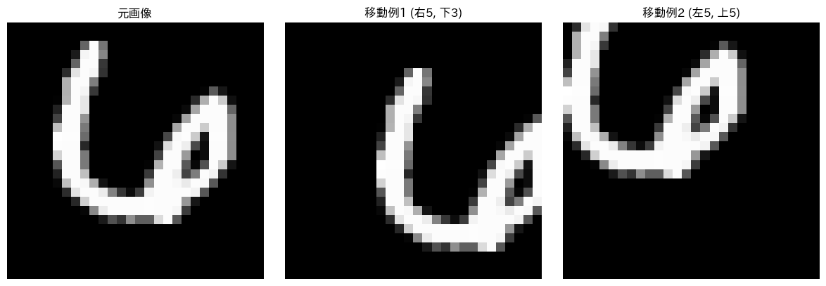
# ===================================================================
# 幾何学的変換:平行移動 (Translation)
# ===================================================================

# 画像のサイズ
(h, w) = original_np_img.shape

# --- 例1: 右に5ピクセル、下に3ピクセル移動 ---
tx1, ty1 = 5, 3
# 2x3の移動行列 [ [1, 0, tx], [0, 1, ty] ] を定義
M1 = np.float32([
    [1, 0, tx1],
    [0, 1, ty1]
])
# cv2.warpAffineで変換を適用
translated_img1 = cv2.warpAffine(original_np_img, M1, (w, h))

# --- 例2: 左に-7ピクセル、上に-7ピクセル移動 ---
tx2, ty2 = -5, -5
M2 = np.float32([
    [1, 0, tx2],
    [0, 1, ty2]
])
translated_img2 = cv2.warpAffine(original_np_img, M2, (w, h))

# 可視化
display_transforms(
    original_np_img,
    [translated_img1, translated_img2],
    [f"移動例1 (右{tx1}, 下{ty1})", f"移動例2 (左{-tx2}, 上{-ty2})"]
)
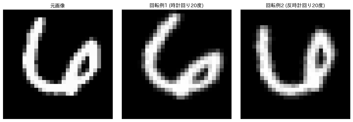
# ===================================================================
# 幾何学的変換:回転 (Rotation)
# ===================================================================

# 画像のサイズと中心座標
(h, w) = original_np_img.shape
center = (w // 2, h // 2)

# --- 例1: 時計回りに15度回転 ---
angle1 = 20
scale1 = 1.0 # 拡大率は1.0に固定
# 回転行列を計算
M1 = cv2.getRotationMatrix2D(center, -angle1, scale1) # -angleで時計回り
# 変換を適用
rotated_img1 = cv2.warpAffine(original_np_img, M1, (w, h))

# --- 例2: 反時計回りに25度回転 ---
angle2 = -20
scale2 = 1.0
# 回転行列を計算
M2 = cv2.getRotationMatrix2D(center, -angle2, scale2) # -(-angle) = +angleで反時計回り
# 変換を適用
rotated_img2 = cv2.warpAffine(original_np_img, M2, (w, h))

# 可視化
display_transforms(
    original_np_img,
    [rotated_img1, rotated_img2],
    [f"回転例1 (時計回り{angle1}度)", f"回転例2 (反時計回り{-angle2}度)"]
)
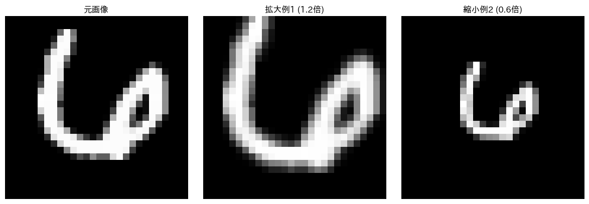
# ===================================================================
# 幾何学的変換:拡大・縮小 (Scaling)
# ===================================================================

# 画像のサイズと中心座標
(h, w) = original_np_img.shape
center = (w // 2, h // 2)
angle = 0 # 回転なし

# --- 例1: 1.2倍に拡大(ズームイン) ---
scale1 = 1.2
# 回転行列を計算 (角度0でスケールのみ適用)
M1 = cv2.getRotationMatrix2D(center, angle, scale1)
# 変換を適用
scaled_img1 = cv2.warpAffine(original_np_img, M1, (w, h))

# --- 例2: 0.8倍に縮小(ズームアウト) ---
scale2 = 0.6
# 回転行列を計算
M2 = cv2.getRotationMatrix2D(center, angle, scale2)
# 変換を適用
scaled_img2 = cv2.warpAffine(original_np_img, M2, (w, h))

# 可視化
display_transforms(
    original_np_img,
    [scaled_img1, scaled_img2],
    [f"拡大例1 ({scale1:.1f}倍)", f"縮小例2 ({scale2:.1f}倍)"]
)
CNNに関する資料,サンプルコード#
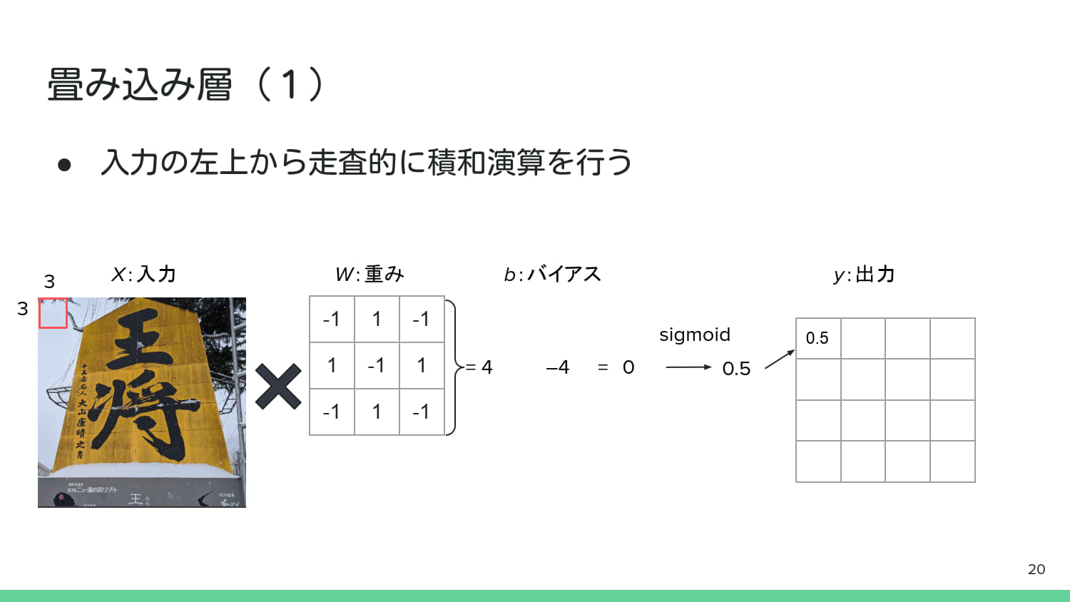
from util import sigmoid
# 入力画像(3x3,P.20の走査範囲を想定)
input_img_p21 = np.array([
[10, 3, 10, 5, 10],
[10, 10, 5, 10, 10],
[10, 7, 10, 3, 10],
[10, 10, 10, 10, 10],
[10, 10, 10, 10, 10]
])
# 重み(カーネル/フィルタ) (3x3,P.20のWを想定)
kernel_p20 = np.array([
[-1, 1, -1],
[1, -1, 1],
[-1, 1, -1]
])
bias_conv = 4 # バイアス (b)
# 畳み込み演算をシミュレーションする関数
def convolution_step(input_region, kernel, bias):
# 積和演算: 入力領域とカーネル(重み)の内積
weighted_sum = np.sum(input_region * kernel)
# バイアスを引く
net_input = weighted_sum - bias
# 活性化関数を適用(ここではSigmoidを想定 - P.20の図より)
output = sigmoid(net_input)
return weighted_sum, output
# 入力画像の左上3x3領域 (P.20の走査範囲)
input_region_p20 = input_img_p21[0:3, 0:3]
# P.20のシミュレーション
sum_p20, output_p20 = convolution_step(input_region_p20, kernel_p20, bias_conv)
print("--- 畳み込み層の動作 (P.20) ---")
print(f"入力領域 (3x3):\n{input_region_p20}")
print(f"カーネル (3x3):\n{kernel_p20}")
print(f"積和: {sum_p20}")
# P.20の計算例では net_input = 0 となり,出力はステップ関数で 1 を想定.
# Sigmoidの場合,0.5に近い値が出力される.
print(f"net_input (積和 - バイアス): {sum_p20 - bias_conv}")
print(f"活性化関数(Sigmoid)出力: {output_p20:.8f}")
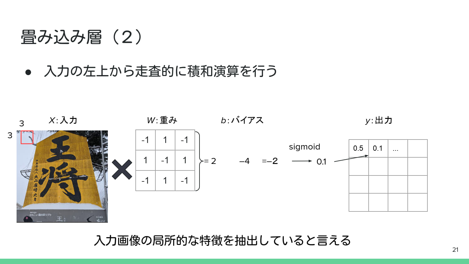
# --- P.21の走査範囲を想定(少し異なるパターン) ---
# P.21の走査範囲(例として,右上2x2が暗いエッジ部分を想定)
# 走査位置を右上に移動 (例: 1行1列目から開始)
input_region_p21 = input_img_p21[0:3, 1:4]
# P.21のシミュレーション
sum_p21, output_p21 = convolution_step(input_region_p21, kernel_p20, bias_conv)
print("\n--- 畳み込み層の動作 (P.21 - 走査位置移動) ---")
print(f"入力領域 (3x3):\n{input_region_p21}")
print(f"積和: {sum_p21}")
# P.21の計算例では net_input = -2 となり,出力はステップ関数で 0 を想定.
print(f"net_input (積和 - バイアス): {sum_p21 - bias_conv}")
print(f"活性化関数(Sigmoid)出力: {output_p21:.8f}")
--- 畳み込み層の動作 (P.20) ---
入力領域 (3x3):
[[10  3 10]
 [10 10  5]
 [10  7 10]]
カーネル (3x3):
[[-1  1 -1]
 [ 1 -1  1]
 [-1  1 -1]]
積和: -25
net_input (積和 - バイアス): -29
活性化関数(Sigmoid)出力: 0.00000000

--- 畳み込み層の動作 (P.21 - 走査位置移動) ---
入力領域 (3x3):
[[ 3 10  5]
 [10  5 10]
 [ 7 10  3]]
積和: 17
net_input (積和 - バイアス): 13
活性化関数(Sigmoid)出力: 0.99999774
CNNを用いてMNISTデータセットの分類を行うサンプルコード#
import torch
import torch.nn as nn
import torch.optim as optim
import torch.nn.functional as F
from torchvision import datasets, transforms
from torch.utils.data import DataLoader

# GPU利用設定
device = torch.device("cuda" if torch.cuda.is_available() else "cpu")
print("使用デバイス:", device)

# データ変換(Tensor化+正規化)
transform = transforms.Compose([
    transforms.ToTensor(),
    transforms.Normalize((0.5,), (0.5,))
])

# MNISTのダウンロード&読み込み
train_dataset = datasets.MNIST(root="./data", train=True, download=True, transform=transform)
test_dataset = datasets.MNIST(root="./data", train=False, download=True, transform=transform)

train_loader = DataLoader(train_dataset, batch_size=64, shuffle=True)
test_loader = DataLoader(test_dataset, batch_size=1000, shuffle=False)
使用デバイス: cuda
# MNISTの画像を10例表示
import matplotlib.pyplot as plt
fig, axes = plt.subplots(4, 5, figsize=(10, 8))
for i, (img, label) in enumerate(test_dataset):
    if i >= 20:
        break
    ax = axes[i // 5, i % 5]
    ax.imshow(img.squeeze(), cmap='gray')
    ax.set_title(f"ラベル: {label}", fontsize=10)
    ax.set_xticks([])
    ax.set_yticks([])
plt.tight_layout()
plt.show()
class SimpleCNN(nn.Module):
    def __init__(self):
        super(SimpleCNN, self).__init__()
        self.conv = nn.Conv2d(1, 8, kernel_size=3, padding=1)  # 1層だけ
        self.fc = nn.Linear(8 * 28 * 28, 10)

    def forward(self, x):
        x = F.relu(self.conv(x))
        x = x.view(x.size(0), -1)
        x = self.fc(x)
        return x

model = SimpleCNN().to(device)
print(model)
SimpleCNN(
  (conv): Conv2d(1, 8, kernel_size=(3, 3), stride=(1, 1), padding=(1, 1))
  (fc): Linear(in_features=6272, out_features=10, bias=True)
)
def train(model, loader, optimizer, criterion):
    model.train()
    total_loss = 0
    for images, labels in loader:
        images, labels = images.to(device), labels.to(device)

        optimizer.zero_grad()
        outputs = model(images)
        loss = criterion(outputs, labels)
        loss.backward()
        optimizer.step()

        total_loss += loss.item()
    return total_loss / len(loader)

def test(model, loader, criterion):
    model.eval()
    correct = 0
    total_loss = 0
    with torch.no_grad():
        for images, labels in loader:
            images, labels = images.to(device), labels.to(device)
            outputs = model(images)
            loss = criterion(outputs, labels)
            total_loss += loss.item()
            pred = outputs.argmax(dim=1)
            correct += pred.eq(labels).sum().item()
    acc = correct / len(loader.dataset)
    return total_loss / len(loader), acc
import matplotlib.pyplot as plt
import seaborn as sns
from sklearn.metrics import confusion_matrix

# 学習履歴を記録するリスト
train_losses, test_losses, test_accs = [], [], []

criterion = nn.CrossEntropyLoss()
optimizer = optim.Adam(model.parameters(), lr=0.001)

# 学習ループ
for epoch in range(5):
    train_loss = train(model, train_loader, optimizer, criterion)
    test_loss, test_acc = test(model, test_loader, criterion)
    train_losses.append(train_loss)
    test_losses.append(test_loss)
    test_accs.append(test_acc)
    print(f"Epoch {epoch+1}: TrainLoss={train_loss:.4f}, TestLoss={test_loss:.4f}, TestAcc={test_acc*100:.2f}%")
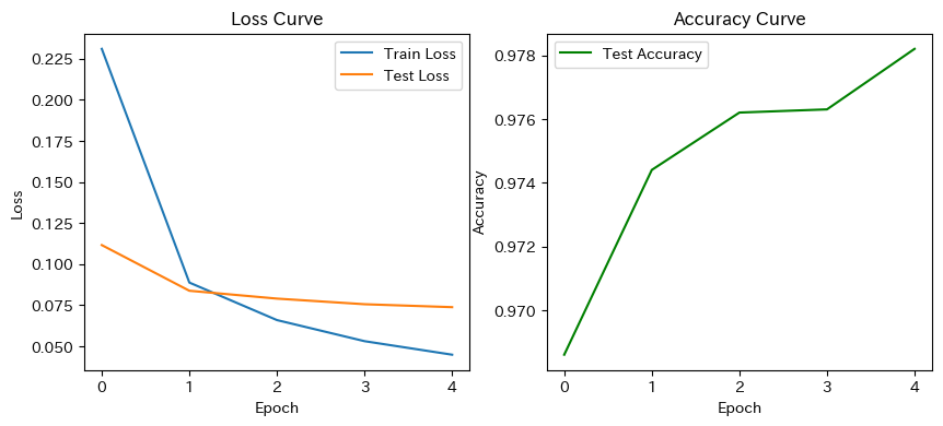
Epoch 1: TrainLoss=0.2310, TestLoss=0.1116, TestAcc=96.86%
Epoch 2: TrainLoss=0.0888, TestLoss=0.0838, TestAcc=97.44%
Epoch 3: TrainLoss=0.0660, TestLoss=0.0790, TestAcc=97.62%
Epoch 4: TrainLoss=0.0531, TestLoss=0.0756, TestAcc=97.63%
Epoch 5: TrainLoss=0.0449, TestLoss=0.0738, TestAcc=97.82%
# 学習曲線の描画
plt.figure(figsize=(10,4))
plt.subplot(1,2,1)
plt.plot(train_losses, label="Train Loss")
plt.plot(test_losses, label="Test Loss")
plt.title("Loss Curve")
plt.xlabel("Epoch")
plt.ylabel("Loss")
plt.legend()

plt.subplot(1,2,2)
plt.plot(test_accs, label="Test Accuracy", color='green')
plt.title("Accuracy Curve")
plt.xlabel("Epoch")
plt.ylabel("Accuracy")
plt.legend()
plt.show()
# 予測例表示
model.eval()
images, labels = next(iter(test_loader))
images, labels = images.to(device), labels.to(device)
outputs = model(images)
preds = outputs.argmax(dim=1)

plt.figure(figsize=(10,4))
for i in range(8):
    plt.subplot(2,4,i+1)
    plt.imshow(images[i].cpu().squeeze(), cmap="gray")
    plt.title(f"P:{preds[i].item()} / T:{labels[i].item()}")
    plt.axis("off")
plt.tight_layout()
plt.show()

# 全テストデータに対して予測
all_preds, all_labels = [], []
model.eval()
with torch.no_grad():
    for images, labels in test_loader:
        images, labels = images.to(device), labels.to(device)
        outputs = model(images)
        preds = outputs.argmax(dim=1)
        all_preds.extend(preds.cpu().numpy())
        all_labels.extend(labels.cpu().numpy())

# 混同行列
cm = confusion_matrix(all_labels, all_preds)
plt.figure(figsize=(8,6))
sns.heatmap(cm, annot=True, fmt="d", cmap="Blues")
plt.title("Confusion Matrix (Simple CNN)")
plt.xlabel("Predicted")
plt.ylabel("True")
plt.show()

# 予測失敗した例の表示
incorrect_indices = [i for i, (p, t) in enumerate(zip(all_preds, all_labels)) if p != t]
plt.figure(figsize=(10,8))
for i, idx in enumerate(incorrect_indices[:16]):
    img, label = test_dataset[idx]
    plt.subplot(4,4,i+1)
    plt.imshow(img.squeeze(), cmap="gray")
    plt.title(f"P:{all_preds[idx]} / T:{label}")
    plt.axis("off")
plt.tight_layout()
plt.show()